
What is A* Algorithm?
“A* (pronounced A-star) is an Informed Search Algorithm used to find the shortest and most efficient path from a start node to a goal node.
It is one of the most powerful search algorithms in Artificial Intelligence.”
A* is a combination of two ideas:
- Uniform Cost Search (which focuses on cost so far)
- Greedy Best-First Search (which focuses on estimated cost to goal)
So A* tries to balance both to reach the goal efficiently.
Why We Need A*
Let’s remind students what happened before:
- In Best-First Search, we only used heuristic (h) → It was fast but not always optimal.
- In Uniform Cost Search, we used only actual cost (g) → It was optimal but slow.
A* solves both problems by combining the two:
f(n)=g(n)+h(n)
Evaluation Function Formula
The core of the A* algorithm is its evaluation function:
f(n)=g(n)+h(n)
Where:
| Symbol | Meaning | Explanation |
| g(n) | Actual cost | Cost from the start node to the current node |
| h(n) | Heuristic (estimated cost) | Estimated cost from the current node to the goal |
| f(n) | Evaluation function | Total estimated cost of the path through node n |
“We use this f(n) to decide which node to expand next — the smaller the f(n), the better the node looks.”
How A* Works (Step-by-Step Logic)
A* Search Algorithm
- Put the start node (S) in the OPEN list.
- If OPEN is empty, stop → no solution.
- Pick the node with the smallest f(n) from OPEN.
- If this node is the goal, stop → solution found.
- Otherwise:
- Move it to the CLOSED list (expanded nodes).
- Generate all its successors.
- For each successor:
- Calculate f(n) = g(n) + h(n)
- Add it to OPEN (if not already there or if f is better).
- Repeat steps 2–5 until the goal is reached.
Important Lists
| List | Meaning |
| OPEN | Nodes discovered but not yet expanded (sorted by f) |
| CLOSED | Nodes already expanded (visited) |
Understanding with an Analogy
“Imagine you’re using Google Maps to go from your home to your college.
- The distance you’ve already travelled is g(n).
- The remaining distance shown by the map is h(n).
- The total travel estimate is f(n) = g + h.
The app always chooses the road with the smallest total travel time (f) — that’s what A* does!”
Example Problem
Problem
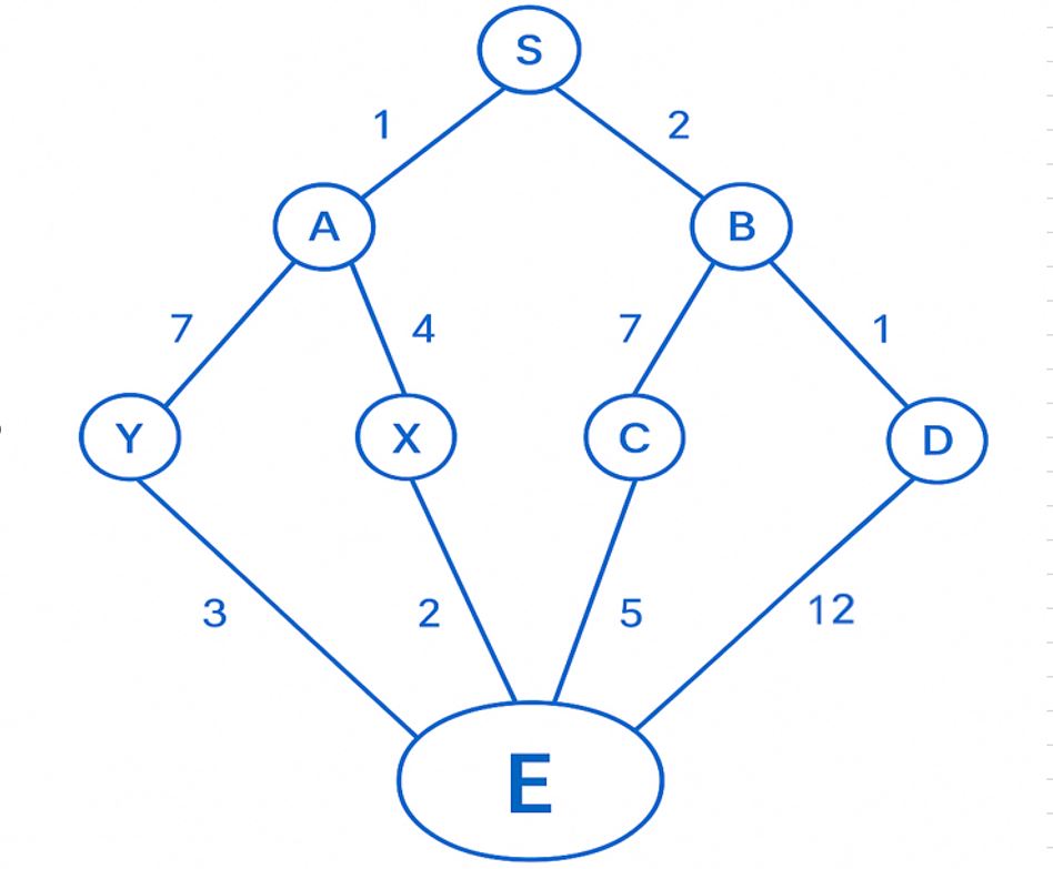
Start = S, Goal = E. Edges (costs on drawing):
- S → A = 1
- S → B = 2
- A → Y = 7
- A → X = 4
- B → C = 7
- B → D = 1
- Y → E = 3
- X → E = 2
- C → E = 5
- D → E = 12
Heuristic values :
h(A) = 5
h(B) = 6
h(C) = 4
h(D) = 15
h(X) = 5
h(Y) = 8
h(E) = 0
We will run A* where f(n) = g(n) + h(n).
g(n) = cost so far from S to n. Start: g(S)=0.
A* Step-by-step
We keep an OPEN (priority queue by lowest f) and a CLOSED set (expanded nodes)..
🔹 Step 1: Initialization
We begin with the start node (S).
At the start:
g(S)=0 ,h(S)=0 (or not considered),
f(S)=g(S)+h(S)= 0,
OPEN list (priority queue) = { S(f=0) }
CLOSED list = { }
We will expand nodes from the OPEN list according to their evaluation function value (f) —
the node with the smallest f is always expanded first.
🔹 Step 2: Expand Start Node (S)
From S, we can move to:
- A with edge cost 1
- B with edge cost 2
Now apply the evaluation function f(n) = g(n) + h(n) for each successor:
| Node | g(n) | h(n) | f(n) = g + h |
| A | 0 + 1 = 1 | 5 | 6 |
| B | 0 + 2 = 2 | 6 | 8 |
✅ OPEN = { A(f=6), B(f=8) }
CLOSED = { S }
Here, f(n) is our evaluation function value.
The smaller f(n), the more promising the node.
So A has f=6 and B has f=8.
Hence, we choose A for expansion next.
🔹 Step 3: Expand Node A (lowest f = 6)
From A, we have two successors:
- Y with edge cost = 7
- X with edge cost = 4
Now compute the evaluation function for each:
| Node | g(n) | h(n) | f(n) = g + h |
| Y | 1 + 7 = 8 | 8 | 16 |
| X | 1 + 4 = 5 | 5 | 10 |
✅ OPEN before inserting new: { B(f=8) }
✅ OPEN after adding: { B(f=8), X(f=10), Y(f=16) }
CLOSED = { S, A }
We now compare the evaluation function values of all available nodes.
The lowest f(n) = 8 for node B,
so node B will be expanded next.
🔹 Step 4: Expand Node B (lowest f = 8)
From B, we have two successors:
- C with edge cost = 7
- D with edge cost = 1
Now calculate their evaluation function values:
| Node | g(n) | h(n) | f(n) = g + h |
| C | 2 + 7 = 9 | 4 | 13 |
| D | 2 + 1 = 3 | 15 | 18 |
✅ OPEN after adding: { X(f=10), C(f=13), Y(f=16), D(f=18) }
CLOSED = { S, A, B }
Now again, we look for the node with the smallest evaluation function value.
Among X(10), C(13), Y(16), and D(18),
the smallest f(n) = 10 (for X).
Hence, X will be expanded next.
🔹 Step 5: Expand Node X (lowest f = 10)
From X, we can move directly to the goal node E with cost = 2.
Now calculate evaluation function for E:
| Node | g(n) | h(n) | f(n) = g + h |
| E | 5 + 2 = 7 | 0 | 7 |
✅ OPEN = { E(f=7), C(f=13), Y(f=16), D(f=18) }
CLOSED = { S, A, B, X }
The evaluation function value for E is f=7,
which is now the smallest among all nodes.
Since E is the goal node, the search stops here.
🏁 Step 6: Path Found
We stop when the goal node is expanded (i.e., taken from OPEN).
Now, trace back the path that led to E:
S→A→X→ES \rightarrow A \rightarrow X \rightarrow ES→A→X→E
✅ Total cost:
g(E)=1+4+2=7g(E) = 1 + 4 + 2 = 7g(E)=1+4+2=7
So, the best path found by the A* algorithm is:
S → A → X → E, with a total cost of 7.
Understanding Why It’s Optimal
- The A* algorithm always expands the node with the lowest evaluation function value.
- The evaluation function balances:
- g(n) → actual cost so far
- h(n) → estimated cost to goal
- This ensures A* doesn’t just take the “closest-looking” path (like Greedy Search)
nor the “cheapest-so-far” path (like Uniform Cost Search).
Instead, it picks the one that seems best overall using both.
In short:
“f(n) = g(n) + h(n) helps the algorithm decide which path is worth exploring next —
balancing both what we already travelled and what we think is left.”
The A* algorithm works based on its evaluation function f(n) = g(n) + h(n).
This function gives each node a score that tells how promising that node is.
- g(n) tells how far we’ve actually come,
- h(n) tells how far we estimate to go,
- and f(n) tells the total estimated effort.
At every step, we expand the node with the smallest f(n).
When the goal node is finally expanded,
we can be sure that we’ve found the best possible path (if h is admissible).