Numerical example of decision tree using ID3
Suppose, we have, 2 features
Feature 1,
(Feature = F1)
Feature

Explanation
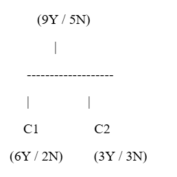
Root Node:
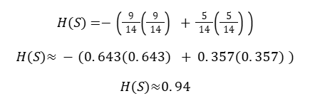
Feature → 9 Yes / 5 No
 First Split (C1):
6 Yes / 2 No → More pure node
 Second Split (C2):
3 Yes / 3 No → Highly impure node
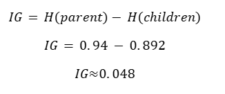
Step 1: Entropy of Root Node
Entropy Formula

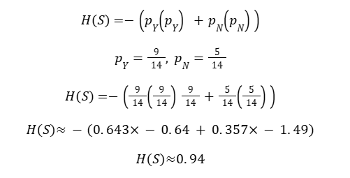
Root node is impure
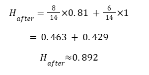
Step 2: Entropy of Child Node C1 (6Y / 2N)

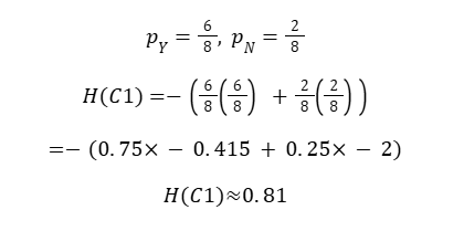
More pure node
Step 3: Entropy of Child Node C2 (3Y / 3N)

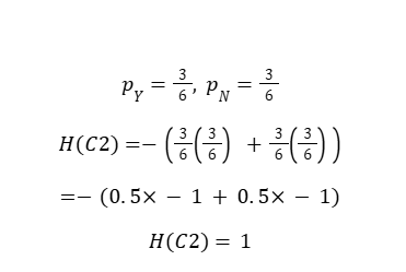
Highly impure node (maximum entropy)
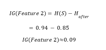
Information gain

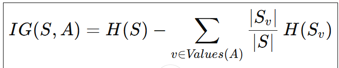
Where:

• → Entire dataset (parent node)
• → Attribute / feature used for splitting
• → All possible values of attribute
• → Subset of where attribute
• → Total number of samples
• → Number of samples in subset
• → Entropy of parent node
  → Entropy of child node

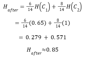
Step 4: Weighted Entropy After Split

Step 5: Information Gain
Formula

(Feature 2)
Root (S): 9Y / 5N → Total = 14
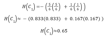
Child C1: 5Y / 1N → Total = 6
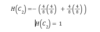
Child C2: 4Y / 4N → Total = 8
Step 1: Entropy of Root Node

Step 2: Entropy of Child C1 (5Y / 1N)

Step 3: Entropy of Child C2 (4Y / 4N)

Step 4: Weighted Entropy After Split

Step 5: Information Gain for Feature 2

Feature 1

• Root: 9Y / 5N
• Children:
• C1 → 6Y / 2N
• C2 → 3Y / 3N

Feature 2
Root: 9Y / 5N
Children:
C1 → 5Y / 1N
C2 → 4Y / 4N

Comparison Table

Feature	Information Gain
Feature 1	≈ 0.05
Feature 2	≈ 0.09

Final Conclusion (ID3 Decision)
ID3 algorithm always selects the feature with the highest Information Gain as the root
node.
Since:

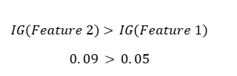
Feature 2 is selected as the ROOT FEATURE