
Choosing the Best Fit Line
Initially:
We start with random values of θ₀ and θ₁
This gives an initial line
However:
So far, we have drawn a straight line to represent the relationship between the independent and dependent variables.
But here comes an important question:
Is the first line we draw always the correct one?
The answer is NO.
When we draw a line initially, it is usually just a guess.
This line may:
- Pass far away from some data points
- Produce large prediction errors
In other words, the predicted values may be very different from the actual values.
The Real Problem
For each data point:
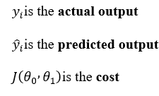
- We have an actual value (y)
- We also have a predicted value (ŷ)
The difference between them is called error.
If the errors are large, the line is not good enough.
So the natural question is:
How can we adjust the line so that the errors become smaller and smaller?
This Is Where Optimization Comes In
Optimization in Linear Regression
So far, we understood that linear regression draws a straight line to fit the data.
However, our initial line is usually not perfect.
To make the line better and better, we need to optimize it.
To get a better fit:
As shown in a diagram, We adjust θ₀ and θ₁ step by step
Each adjustment reduces the prediction error
This process is called optimization.
The goal is:
To make the line fit the data better and better until error is minimized.
Final Goal of Optimization
The final aim is:
- To find θ₀ and θ₁ Such that the regression line gives minimum error for all data points
This leads to the best fit line.
What Are We Optimizing?
In linear regression, the equation is:
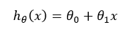
To improve the line, we optimize:
θ₀ (intercept)
θ₁ (slope)
By changing these values, we get different straight lines.
Why Do We Need Optimization?
Because:
There are many possible straight lines
We must choose the best fit line
The best fit line is the one with minimum error
So, we need a way to measure how bad or good a line is.
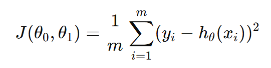
Cost Function (Loss Function)
To measure the error of a line, we use a cost function.
The cost function tells us:
How much error the model is making for given values of θ₀ and θ₁.
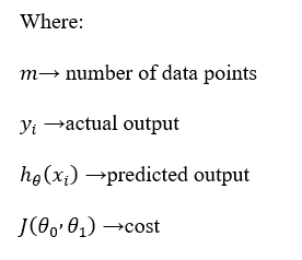
Cost Function for Linear Regression
The cost function used in linear regression is Mean Squared Error (MSE).
Where:
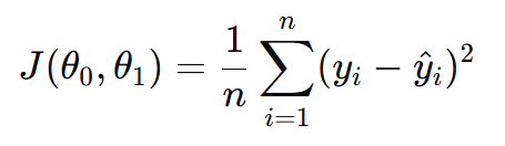
Can be written as
Why Square the Error?
If we simply add errors:
Positive and negative errors may cancel each other
We may wrongly get zero error
So, we square the error:
Makes all errors positive
Penalizes larger errors more
Meaning of the Cost Function
- The cost function calculates the average of squared errors
- Smaller value of cost → better fit
- Larger value of cost → poor fit
👉 Our aim is to minimize this cost function.
Why Is It Called “Mean Squared Error”?
Squared → because we square the error to avoid negative values
Mean → because we take the average of errors for all data points
So,
Mean Squared Error = Mean of (Actual − Predicted)²
Loss Function vs Cost Function
Loss Function
Calculates error for a single data point
Formula:
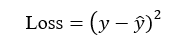
Cost Function
Calculates average loss for all data points
Used to evaluate the entire model
👉 In short:
Loss function → one data point
Cost function → all data points
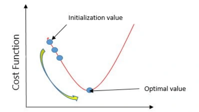
Gradient Descent: Minimizing the Cost Function
From the cost function discussion, we know that our goal is to minimize the cost function J1.
If we plot the cost function against the parameters, we usually get a parabolic (U-shaped) curve.
- The lowest point of this curve represents the global minimum
- At this point, the error is minimum
- This gives us the best fit line
Why Do We Need Gradient Descent?
We cannot directly guess the values of θ₀ and θ₁ that give minimum cost
So, we use an iterative optimization algorithm
This algorithm slowly moves towards the global minimum
This algorithm is called Gradient Descent.
Idea Behind Gradient Descent
Gradient Descent works like this:
Start with initial (random) values of parameters
Calculate the slope (gradient) of the cost function
Move parameters in the opposite direction of the slope
Repeat this process until the minimum cost is reached
This repeated process is called convergence.
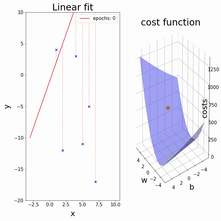
GIF shows how linear regression learns using gradient descent.
- The left graph shows data points and a straight line.
- The right graph shows the cost function surface.
- As training progresses, the line changes its position.
- At the same time, the cost value decreases.
- Finally, the line becomes the best fit line when cost is minimum.
Understanding Gradient Descent Using the Cost Curve (As in the Diagram)
When we plot the cost function Jon the Y-axis and the parameter on the X-axis, we obtain a U-shaped (parabolic) curve.
- The lowest point of this curve represents the global minimum.
- At this point, the cost is minimum.
- Our main goal is to reach this global minimum.
Gradient Descent helps us move step by step toward this minimum point.
Using Tangent and Slope (From the Diagram)
At any point on the curve, we draw a tangent line.
The slope of the tangent tells us the direction in which the cost is changing.
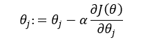
This slope is used to update the value of .
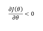
Case 1: Left Side of the Global Minimum
When the current point lies on the left side of the global minimum:
- The cost curve is sloping downward
- The slope of the tangent is negative
Mathematically:
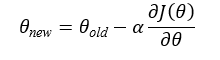
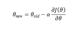
Gradient Descent Update Rule
The gradient descent update rule is:
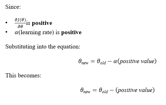
What Happens When the Slope Is Negative?
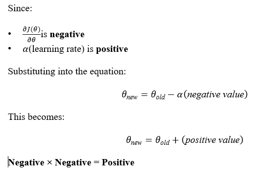
➡️ Negative × Negative = Positive
Effect on Parameter Value
- The value of increases
- The point moves to the right on the cost curve
- This movement is towards the global minimum
Final Intuition
When we are on the left side of the minimum, the slope is negative.
Gradient descent subtracts this negative slope, which effectively adds to the parameter value, moving it closer to the global minimum.
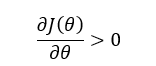
Case 2: Right Side of the Global Minimum
When the current point lies on the right side of the global minimum:
- The cost curve is sloping upward
- The slope of the tangent is positive
Mathematically:
Gradient Descent Update Rule
The gradient descent update rule is:
What Happens When the Slope Is Positive?
Effect on Parameter Value
- The value of decreases
- The point moves to the left on the cost curve
- This movement is towards the global minimum
Final Intuition
When we are on the right side of the minimum, the slope is positive.
Gradient descent subtracts this positive slope, which reduces the parameter value and moves it closer to the global minimum.
| Position | Slope | Update Effect | Direction | Result |
| Left of minimum | Negative | − (− value) = + | Move right | Towards minimum |
| Right of minimum | Positive | − (+ value) = − | Move left | Towards minimum |
Effect of Learning Rate in Gradient Descent
From the gradient descent update rule:
we can clearly see that learning rate (α) plays a very important role.
Why Gradient Descent Converges
Each update moves in the direction of decreasing cost
With repeated updates, the cost value reduces slowly
Eventually, the algorithm reaches the global minimum
This gradual movement is called convergence.
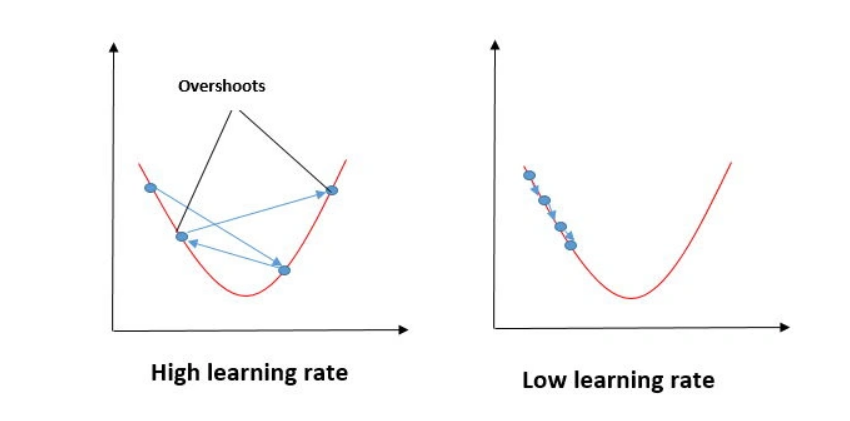
What If Learning Rate Is Too Large?
If α is very large:
Parameter updates become very big
The algorithm may jump over the minimum
It may oscillate back and forth
The model may never reach the global minimum
In such cases:
Gradient descent fails to converge.
What If Learning Rate Is Too Small?
If α is very small:
Updates become very slow
Convergence takes a long time
Model still reaches minimum, but very slowly
So:
Small α = safe but slow learning
Choosing the Right Learning Rate
Learning rate controls the speed of convergence
It should be:
Not too large (to avoid overshooting)
Not too small (to avoid slow learning)
Hence:
Learning rate should be a small positive value
Default Learning Rate
In many practical implementations:
A small value like

is used as a default learning rate
This value usually provides a good balance between:
Speed of convergence
Stability of learning
Gradient Descent as a Convergence Algorithm
Gradient Descent is called a convergence algorithm because:
- It gradually reduces the cost function
- With each iteration, parameters move closer to the minimum
- Finally, it reaches the global minimum
At this point:
- The cost function becomes minimum
The regression model becomes optimal