
CBOW is one of the two ways to train Word2Vec.
Simple Example
Sentence:
NLP NAME IS RELATED TO DATA SCIENCE
steps:
Step 1: Data Preparation
- Take text corpus:
NLP NAME IS RELATED TO DATA SCIENCE
- Tokenize into words.
- Build vocabulary (unique words):
[NLP, NAME, IS, RELATED, TO, DATA, SCIENCE]
consider
- Fix window size = 5.
Step 2: Generate Context–Target Pairs
Choose a window size (say 5).
For every word:
- Take surrounding words → Context
- Middle word → Target
Suppose, Window Size = 5
Window size = 5 means:
- 2 words from left
- 1 target word (middle)
- 2 words from right
So total = 5 words.
IS is chosen as the target word.
Highlighted:
NLP NAME [IS] RELATED TO
Example:
Input and Output
🟢 Input (Context Words):
Take all words except IS inside the window:
[NLP, NAME, RELATED, TO]
🟡 Output (Target):
IS
So CBOW learns:
NLP + NAME + RELATED + TO → IS
Sliding Window
Next, the window moves forward:
NAME IS RELATED TO DATA
Now:
Input:
[NAME, IS, TO, DATA]
Output:
RELATED
So:
NAME + IS + TO + DATA → RELATED
These pairs are created for the entire corpus.
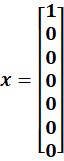
Step 3: One-Hot Encoding
Each word is converted into a vector based on vocabulary.
Example:
NLP → [1 0 0 0 0 0 0]

NAME    → [0 1 0 0 0 0 0]

IS      → [0 0 1 0 0 0 0]
These are input representations.
Step 3: Build the CBOW Model Architecture
It contains:
- Input layer (context words)
- Hidden layer (embedding layer)
- Output layer (target word)
The hidden layer weights become the word embeddings.
CBOW Model Architecture is as shown in the figure,
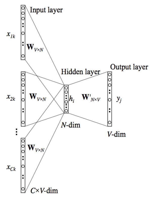
CBOW Architecture
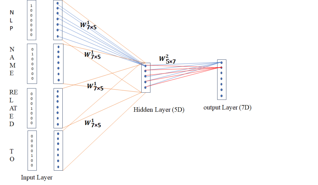
CBOW Architecture as per our example
1. Input Layer :
Each context word is first converted to one-hot vectors.
Vocabulary (7 words):
[NLP, NAME, IS, RELATED, TO, DATA, SCIENCE]
So one-hot vectors are:
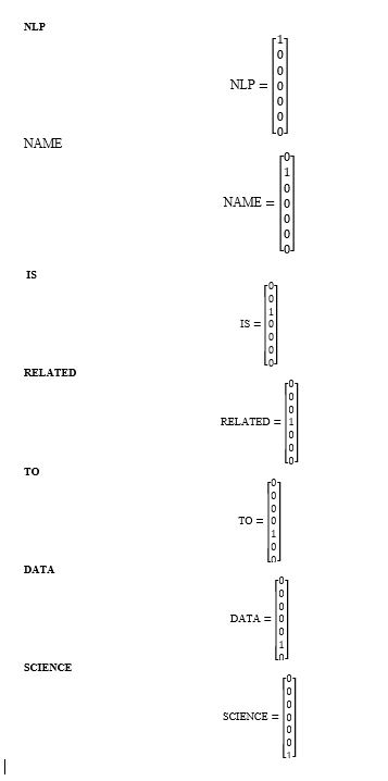
Only context words are used as input.
- Embedding Layer / Hidden Layer (Middle Block – 7×5)
Here, size is 7 × 5
Meaning:
- Vocabulary size = 7
- Embedding dimension = 5
So we create a weight matrix W (7×5):
W =
So original

must look like:
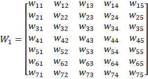
Initially random.
How one-hot becomes dense
Hidden Layer Computation
Hidden size:

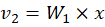
Since input is

and W is

We compute hidden vector as:


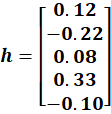
And it becomes:
So:
So, h = 51
Example weight matrix(w1):
| Word | e1 | e2 | e3 | e4 | e5 |
| NLP | 0.12 | -0.22 | 0.08 | 0.33 | -0.10 |
| NAME | -0.21 | 0.34 | 0.11 | 0.52 | -0.08 |
| IS | 0.23 | -0.41 | 0.67 | 0.32 | 0.45 |
| RELATED | 0.09 | 0.55 | -0.12 | 0.14 | 0.26 |
| TO | -0.14 | 0.33 | 0.21 | -0.09 | 0.18 |
| DATA | … | ||||
| SCIENCE | … |
Initially random.
So

| NLP | NAME | IS | RELATED | TO | DATA | SCIENCE | |
| e1 | 0.12 | -0.21 | 0.23 | 0.09 | -0.14 | … | … |
| e2 | -0.22 | 0.34 | -0.41 | 0.55 | 0.33 | … | … |
| e3 | 0.08 | 0.11 | 0.67 | -0.12 | 0.21 | … | … |
| e4 | 0.33 | 0.52 | 0.32 | 0.14 | -0.09 | … | … |
| e5 | -0.10 | -0.08 | 0.45 | 0.26 | 0.18 | … | … |
🔶 Input (NLP)
🔷 Hidden Calculation

Matrix rule:
Now compute each row one by one.
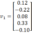
🔹 First Hidden Neuron (Row 1)
Row 1:

Multiply with x:


Second Hidden Neuron (Row 2)
Row 2:

Multiply:


🔹 Third Hidden Neuron
🔹 Fourth Hidden Neuron
🔹 Fifth Hidden Neuron
🔷 Final Hidden Vector
Column 1 of W₁ is selected.
So, Case 1:NLP
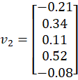
🔷 Case 2: Input = NAME

Multiply:
Selects column 2:

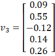
🔷 Case 3: Input = RELATED
Select column 4:

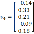
🔷 Case 4: Input = TO
Select column 5:
What We Now Have


Each is:

Each is a dense vector.
From Step 2, we obtained:


Each vector is:

✅ STEP 3 — Context Aggregation (Averaging)
Now CBOW averages them:
Context Vector = (v1 + v2 + v3 + v4) / 4
Let’s calculate element-wise:
First dimension:
(0.12 + (-0.21) + 0.09 + (-0.14)) / 4
= (-0.14) / 4
= -0.035
Second dimension:
(-0.22 + 0.34 + 0.55 + 0.33) / 4
= 1.00 / 4
= 0.25
Third dimension:
(0.08 + 0.11 + (-0.12) + 0.21) / 4
= 0.28 / 4
= 0.07
Fourth dimension:
(0.33 + 0.52 + 0.14 + (-0.09)) / 4
= 0.90 / 4
= 0.225
Fifth dimension:
(-0.10 + (-0.08) + 0.26 + 0.18) / 4
= 0.26 / 4
= 0.065
This gives ONE vector:
Final Context Vector:
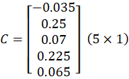
This is the context meaning vector.
This single vector goes to output layer.
All context embeddings are 5×1 column vectors.
We add them element-wise and divide by 4.
The result is a single 5×1 vector called the context vector.
This vector represents the combined meaning of all context words.
This has 5 values
STEP 4 — Output Layer (Prediction)
Output:

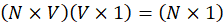
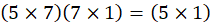
So,:
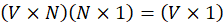
(75)(5
1)=(7
1)
So, output will be of 71
Remember:
Vocabulary = 7 words:
NLP, NAME, IS, RELATED, TO, DATA, SCIENCE
So output layer has:
👉 7 neurons
Each neuron represents one word.
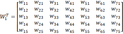
Hidden → Output Weight Matrix(w2)
Suppose w2 is What Does W₂ Look Like (5×7)?
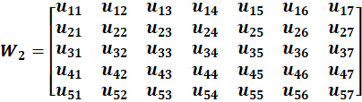
Now the network has another matrix:
Size = 5 × 7
Why?
- 5 inputs (from hidden layer)
- 7 outputs (vocabulary)
- Then W₂ᵀ Becomes (7×5)

Example matrix (w2) (simplified):
| NLP | NAME | IS | RELATED | TO | DATA | SCIENCE | |
| h1 | 0.20 | -0.10 | 0.30 | 0.05 | -0.02 | 0.01 | -0.03 |
| h2 | -0.15 | 0.25 | 0.40 | -0.10 | 0.02 | 0.01 | 0.05 |
| h3 | 0.10 | 0.05 | 0.35 | 0.08 | -0.01 | 0.02 | 0.01 |
| h4 | 0.05 | -0.02 | 0.45 | 0.06 | 0.01 | -0.01 | 0.02 |
| h5 | -0.01 | 0.03 | 0.20 | 0.04 | 0.01 | 0.00 | 0.01 |
So

is
| h1 | h2 | h3 | h4 | h5 | |
| NLP | 0.20 | -0.15 | 0.10 | 0.05 | -0.01 |
| NAME | -0.10 | 0.25 | 0.05 | -0.02 | 0.03 |
| IS | 0.30 | 0.40 | 0.35 | 0.45 | 0.20 |
| RELATED | 0.05 | -0.10 | 0.08 | 0.06 | 0.04 |
| TO | -0.02 | 0.02 | -0.01 | 0.01 | 0.01 |
| DATA | 0.01 | 0.01 | 0.02 | -0.01 | 0.00 |
| SCIENCE | -0.03 | 0.05 | 0.01 | 0.02 | 0.01 |
These values are learned during training.
Multiply Context Vector with this Matrix
Context vector:

Now compute score for each word.
Let’s calculate only IS (because that’s our target).
🧮 IS column calculation
Multiply element-wise and sum:
(-0.03 × 0.30)
+ (0.25 × 0.40)
+ (0.07 × 0.35)
+ (0.22 × 0.45)
+ (0.06 × 0.20)
Step-by-step:
-0.009
+0.100
+0.0245
+0.099
+0.012
Total:
≈ 0.226
This is IS raw score.
Same calculation happens for:
NLP
NAME
RELATED
TO
DATA
SCIENCE
Giving:
NLP → 0.02
NAME → 0.04
IS → 0.226 ⭐
RELATED → 0.05
TO → 0.01
DATA → 0.00
SCIENCE → 0.01
These are called logits.
Important:
👉 These are NOT probabilities yet.
They do NOT sum to 1.
STEP 5 — Softmax (Convert to Probabilities)
What Softmax Does
Softmax converts these raw numbers into probabilities between 0 and 1.
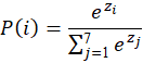
Formula:
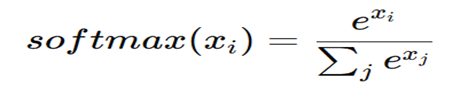
In our example,
Now we convert logits into probabilities.
STEP 1 — Take exponent (e^x)
We compute e^score for each:
| Word | Score | e^score |
| NLP | 0.02 | 1.020 |
| NAME | 0.04 | 1.041 |
| IS | 0.226 | 1.254 |
| RELATED | 0.05 | 1.051 |
| TO | 0.01 | 1.010 |
| DATA | 0.00 | 1.000 |
| SCIENCE | 0.01 | 1.010 |
(Values rounded)
STEP 2 — Add all exponent values
Total = 1.020 + 1.041 + 1.254 + 1.051 + 1.010 + 1.000 + 1.010
Total ≈ 7.386
STEP 3 — Divide each by total
Now probability for each word:
NLP
1.020 / 7.386 ≈ 0.13
NAME
1.041 / 7.386 ≈ 0.14
IS ⭐
1.254 / 7.386 ≈ 0.17 ← highest
RELATED
1.051 / 7.386 ≈ 0.14
TO
1.010 / 7.386 ≈ 0.13
DATA
1.000 / 7.386 ≈ 0.13
SCIENCE
1.010 / 7.386 ≈ 0.13
STEP 6 — Loss Calculation
The model compares:
- Actual word: IS
- Predicted probability for IS: 0.17
- The model is saying:
- “I am only 17% confident that IS is correct.”
- That is very low confidence.
- Model needs correction.
STEP 7 — Backpropagation
Now the error signal is strong because:
Correct word probability = 0.17
But ideal probability should be close to 1.
Now the network asks:
Why did I make this error?
So error flows backward:
Output layer → Hidden layer → Embedding matrix
This adjusts:
- Hidden → output weights
- Input → hidden weights (embedding matrix)
What exactly gets updated?
Remember:
- Embedding matrix (5×7)
- Output weight matrix (7×5)
Both are updated slightly.
Before update:
IS → 0.17 ❌ (too small)
After many updates:
IS → 0.60
Then → 0.80
Then → 0.95
Loss gradually decreases.
STEP 8 — Repeat for All Windows
Same process for:
- IS
- RELATED
- TO
- DATA
- SCIENCE
Over thousands of sentences.
Over many epochs.
Meaning:
1. “Repeat for All Windows”
Remember CBOW uses a sliding window.
Sentence:
NLP NAME IS RELATED TO DATA SCIENCE
Window size = 5
So training examples become:
Window 1:
NLP NAME IS RELATED TO
Target = IS
Window 2:
NAME IS RELATED TO DATA
Target = RELATED
Window 3:
IS RELATED TO DATA SCIENCE
Target = TO
So CBOW does:
- Predict IS
- Update weights
- Predict RELATED
- Update weights
- Predict TO
- Update weights
That is:
👉 Repeat for all windows in the sentence.
✅ 2. “Over Thousands of Sentences”
Not just one sentence.
Model trains on:
- books
- articles
- Wikipedia
- news
Millions of sentences.
Each sentence produces many windows.
So learning becomes strong.
✅ 3. “Over Many Epochs”
Epoch means:
👉 One full pass over entire dataset.
If you train:
- 1 epoch → read all data once
- 5 epochs → read all data 5 times
- 10 epochs → read all data 10 times
Each time:
- predictions improve
- embeddings become better
Simple analogy
Studying:
- Read book once → little learning
- Read book many times → strong memory
Same for model.