Structure of a Neural Network

Okay, now that we’ve met our single artificial neuron — the perceptron — let’s see what happens when many of them start working together.
Think of it like a group project: one neuron alone can do only simple tasks, but when hundreds of them join forces, they can solve complex problems like recognizing faces, understanding speech, or even driving cars! 

A Neural Network is simply a collection of many interconnected neurons arranged in layers.

Definition

“A Neural Network is a computer system made of many artificial neurons (tiny mathematical functions) that work together to learn patterns from data.”

The Three Layers of a Neural Network

1. Input Layer
   This is where the network receives data.
   Each node (or neuron) in this layer represents one feature from the dataset.
   Example: If you are predicting whether an image is of a cat or dog, each pixel’s value from the image becomes an input.
2. Hidden Layer(s)
   This is the brain of the network.
   It processes the inputs, detects patterns, and learns relationships between data.
   The more hidden layers a network has, the deeper it becomes — that’s why we call them Deep Neural Networks (DNNs).
   Example: In our cat-dog image, the first hidden layer might detect edges, the next one eyes and ears, and another might detect fur patterns.
3. Output Layer
   This is where the final decision is made.
   Example: Output layer might say — “ 90% Dog,  10% Cat.”

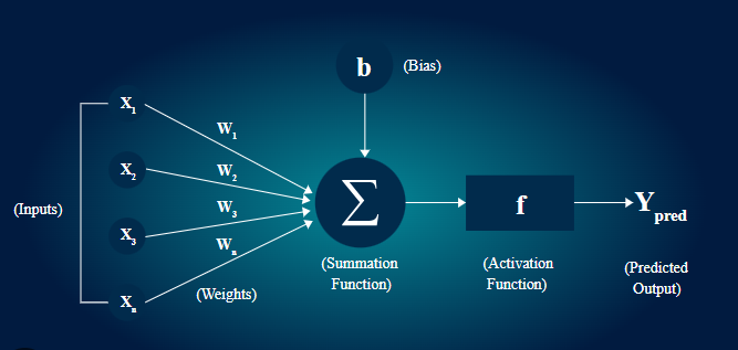
Each connection has a weight (importance), and the network learns by adjusting those weights .

Weights and Bias in neural network

Step-by-Step: How the Learning Happens

1. Input Stage (Getting the Data)
   Everything starts when we feed input data into the network.
   Each input is multiplied by a weight — a number that shows how important that input is.
   For example, if “hours studied” is more important than “hours slept,” it will have a higher weight.
2. Summation (Mixing the Inputs)
   The neuron adds up all the weighted inputs — kind of like combining ingredients in a recipe .
   Each neuron decides what to do with that mix next.
3. Activation Function (Decision Time!)
   Now comes the activation function, which decides whether the neuron should “fire” (activate) or stay quiet.
   It’s like a switch that says, “Yes, this pattern looks important — pass it on!”
4. Output (Making a Prediction)
   The final layer gives the network’s prediction — it could be “Pass” or “Fail,” “Cat” or “Dog,” “Spam” or “Not Spam.”
5. Error Calculation (Oops! That’s Wrong 😅)
   The network then compares its output with the correct answer.
   The difference between them is called Error.
6. Backpropagation (Learning from Mistakes)
   This is the magical part! 🪄
   The network sends the error backward through all the layers and adjusts the weights.
   The next time it makes a slightly better guess.
   Over many rounds (called epochs), the network becomes smarter and more accurate.

---

 In Short

A Neural Network learns by repeating three steps:
Guess → Check → Correct.
This simple cycle is the heart of deep learning! 

how a neural network learns (forward + backward) using simple addition, multiplication, and adjustment — no gradients or calculus.

 Step-by-Step Explanation (Simple Version)

1️⃣ Input features
Tell them:

“Imagine we are trying to teach a neural network to recognize cats.
We give it three features:

• Has whiskers (1 = yes, 0 = no)
• Has pointy ears (1 = yes, 0 = no)
• Has fur (1 = yes, 0 = no)”

Example input:
[1, 1, 1] → means yes, it has whiskers, ears, and fur.

Neural Network Learning Example (Cat or Not Cat)

We’ll use:

• 3 input features
• 1 output neuron
• 1 training example

We want the network to learn whether an image is a cat (1) or not a cat (0).

Feature	Description	Value
x₁	Has whiskers	1
x₂	Has pointy ears	1
x₃	Has fur	1

2️⃣ Initialize weights randomly

Let the initial weights and bias be:

w₁ = 0.2,   w₂ = 0.3,   w₃ = 0.1,   bias = 0.1

3️⃣ Forward pass (prediction)

Compute weighted sum (z):

z=w1+w2+w3+bias

z=1×0.2+1×0.3+1×0.1+0.1=0.7

Now apply sigmoid activation to get a probability:

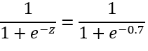
output=11+e-z=11+e-0.7≈0.668

So, the network says:

“This looks 66.8% like a cat.”

4️⃣ Compare with actual label

Actual answer = 1.
Predicted = 0.668.

Error=Target–Output=1-0.668=0.332

So, the network is off by 0.332 (33.2%).

5️⃣ Weight update (simple learning rule)(Backward pass)

We use a simple rule:

New weight=Old weight+Learning rateErrorInput

Let learning rate η = 0.1

Then:

w1=0.1×0.332×1=0.0332

w2=0.1×0.332×1=0.0332

w3=0.1×0.332×1=0.0332

b=0.1×0.332=0.0332

6️⃣ Update all weights

w1=0.2+0.0332=0.2332

w2=0.3+0.0332=0.3332

w3=0.1+0.0332=0.1332

b=0.1+0.0332=0.1332

7️⃣ Test again (after learning)

Now, compute again:

z=1×0.2332+1×0.3332+1×0.1332+0.1332=0.8328

Output=11+e-0.8328=0.6969

Now the network says:

“I’m 69.7% sure this is a cat (up from 66.8%)!”

Conclusion

Step	Output	Error
Before training	0.668	0.332
After 1 update	0.697	0.303

With more training examples, and many such updates, the network will keep adjusting until it predicts near 1.0 for cats and 0.0 for not-cats.

Key points

• Neural networks never know the correct answer at the start.
• The initial output is just a guess, based on initial random weights.
• Training (forward + backward propagation) is what improves the guess.

So yes, even though all features are “1,” the network outputs 0.668 instead of 1 — this is normal and expected.
It is not wrong, it just shows the network needs training.